How to use?
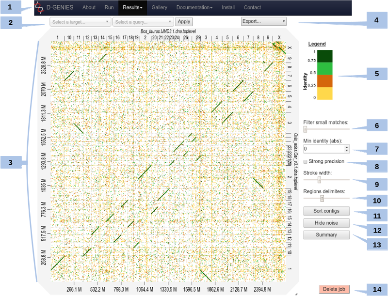
The result page (see above) presents the dot plot following the fasta files sequence order*. The alignment matches are presented as colored lines on the graphical panel. The colors correspond to similarity values (called here identity values) that have been binned in four groups (less than 25%, between 25 and 50%, between 50 and 75% and over 75% similarity).
The top and right margin of the graphical panel show the sequence names. Depending on the sequence and name length, the names will be fully or partially presented. In order to ease visualization, all sequences smaller than 0.2 percent of the total length are merged in a unique super-sequence for which the margin is grayed. The left and bottom margins show the sequence size scales.
* Except if more than 75% of the query length if composed of contigs with size less than 1% of the query length. In this case, contigs of the query are already sorted according to the reference.
(1) Main menu
You can access to your previous results by clicking on the main menu in the Results item. A list will appear with all jobs you have launched on the server.
(2) Select query and target
You can zoom on the graph by pushing the CRTL key while turning the mouse wheel forward to zoom in and backward to zoom out. Drag and drop to move the graph (with CTRL key still pushed).
You can zoom to a specific zone on the graph by clicking on the dotplot. This will zoom into the associated rectangle formed by the query-target contigs association.
Or, you can select the zone by selecting a query and a target in the dropdown menus at the top, and click Apply.
To come back to the initial view, click on the icon at the top right of the dotplot or press ESC.
(3) Matches details
For each match, you can view positions on query and on target and the precise identity value by placing mouse cursor over it.
Due to technical limits, it doesn't work for too small matches. You can zoom to make it work for them.
(4) Export
Several export options are available:
- Export as image (SVG or PNG - suitable for publication). All changes applied to the dot plot will be kept on export, including zoom.
- Download the PAF file generated by minimap2.
- Download the association table: TSV file with, for each contig of the query, the associated chromosome of the target with position of the match (see definitions and documentation about formats for details).
- List of contigs of the query which have no match with any chromosome of the target.
- List of chromosomes of the target which have no match with any contig of the query.
- Export the job as a tar file which can be re-uploaded in the run form to restore the job.
And, if you sorted the dotplot:
- Download the Fasta query file with contigs in the same order as in the dotplot.
- Download all contigs of the query assembled like the chromosomes of the target. We take the diagonal match line, and for all contigs that match the same chromosome, we stick them together, separated by a 100-N block.
(5) Color scheme
You can change the default color scheme. Five other color schemes are available:
- Colorblind colors: colors more distinguishable for colorblind people.
- Black & White: for black & white printing.
- Reverse default: default colors but colors with the lower mapping identity have the lower brightness.
- Reverse Coloblind: same as reverse default, but with colorblind colors.
- All black: all in black.
To change color scheme, click on the legend.
(6) Match size filtering
You can remove too small matches by moving the slider. By increments, it remove matches with size of 0.001 to 0.2% of the dotplot width. Too small matches are also removed by the Remove noise button (see below).
(7) Match identity filtering
Set the minimal identity to show. All matches with a lower identity value will be hidden.
(8) Strong precision
When checked, the strong precision check-box reduces match borders removing small matches from the graphical panel, often showing gaps between non contiguous matches.
(9) Line breadth
Change the match lines thickness with the slider.
(10) Chrom. border breadth
Change the visibility of the chromosomes borders with the slider.
(11) Sort
You can sort (or unsort) contigs by clicking on the button. Contigs of the query will be sorted according to the reference. It will take few seconds.
How it works? For each contig of the query we search the region which have the biggest matches with the target and store these coordinates. Then, we sort contigs by their associated coordinates.
(12) Hide noise
To remove noise. A match is considered noise if its size is small and its size frequency is quite high. Therefore we group matches by size bins, the number of bins corresponds to one tenth of the number of alignments, the bins are scanned in increasing size order to find the most represented one and from this one the one corresponding to one percent of its count is searched. All the alignments in bins smaller in size than this one are considered noise. It will take few seconds.
(13) Similarity summary
To ease dot plot comparison, clicking the summary button generates a bar graph presenting the reference similarity profile, meaning the sums of the projections of the matches on the reference per similarity category divided by the total reference length. This graph is produced after sorting the query along the reference, removing included matches and noise filtering; result not shown on the graphical panel. It gives a realistic view of the overall reference and query similarity which is often not very precisely measured through visual inspection.
(14) Delete job
By clicking on the button, your job will be definitively removed on the server. Be careful, this operation can not be undone!